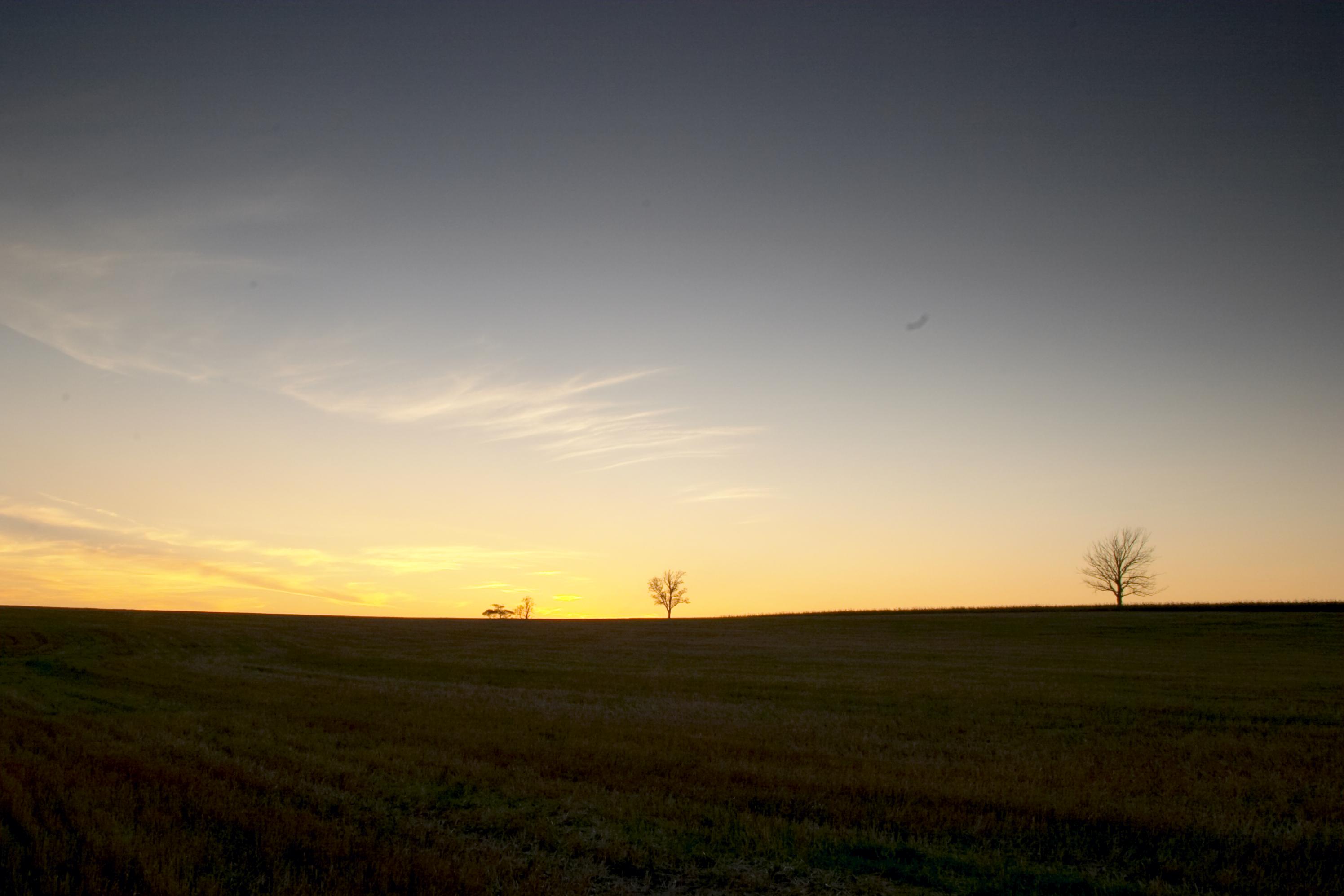
JPEG Version of Original Image
Adjusted image with bands
Frank Bayley compained on the DPREVIEW site about a certain category of pictures that is giving him problems. These images have large areas of gradients of color.
This page serves as an exploration of the cause of the banding and is not intended to be a final explanation. All images are rather large so will be illustrated using small versions, either sized down or cropped. The pictures will also include a link to a full-sized picture that can be used for further inspection. These additional files have been saved as JPEGs because of bandwidth considerations. However, enough information is given for the reader to duplicate the uncompressed files if desired.
JPEG Version of Original Image |
Adjusted image with bands |
Here is the workflow used to produce the image on the right:
The images were shot at ISO 100 (which I use wherever possible) with my EF 20mm f/2.8 USM. My basic workflow, represented in the images, is:
If I do a G/blur fix, (or add noise, or whatever else to knock the radials back) it's usually after Step #5, although in some cases I'll do it after Step #8.
I've been experimenting with doing some of the work in Lab Colour mode (RGB 24-bit), but this has had no positive effect: The gradient banding is still there; same degree.
Just to re-mention one small point, this "only" appears to happen when shooting in RAW; fine jpeg is almost always clean, or at the very least significantly less evident.
For my jpeg workflow Step #1 obviously doesn't happen, and Step #2 is: Open as RGB 24-bit, Adobe-RGB > save as TIFF 48-bit > Step #3 and onward.
Cheers
Frank B.
Ontario CANADA
Following are my suggestions:
First, it looks like Frank is trying to increase the saturation, mainly of the blue.
Next, it must be recognized that the eye can distinguish much finer gradations of color when they are presented in large swaths of neighboring values. Consequently, it's desireable to do as much processing using the original raw file as possible.
For my attempt, I decided to use Breeze Browser. I used the following settings:
Then I used Photoshop 6 to adjust levels, and saturation until I'd approximated the colors in the above image on the right. The result is shown here:
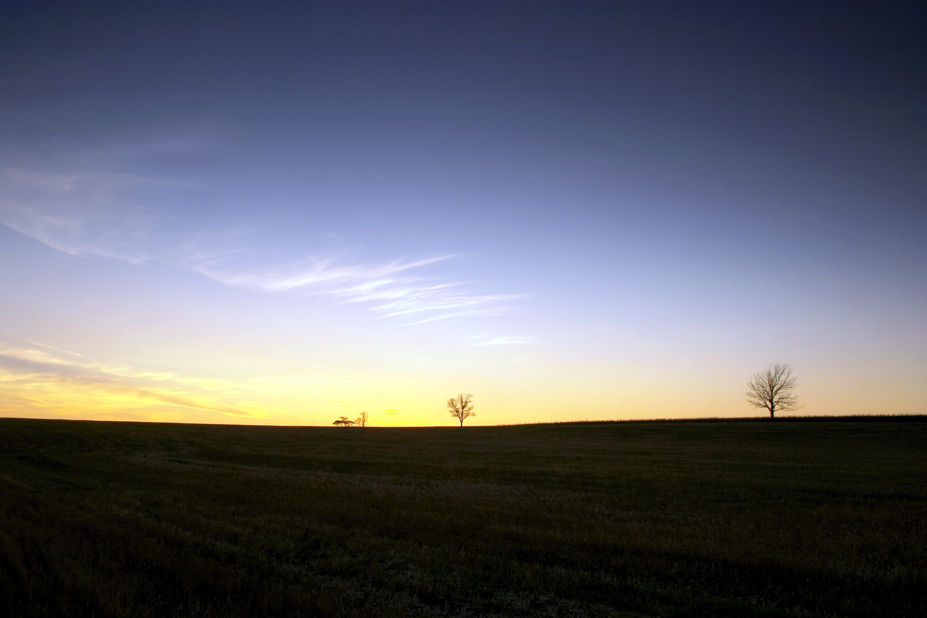
Frank's version of image |
 My version of image |
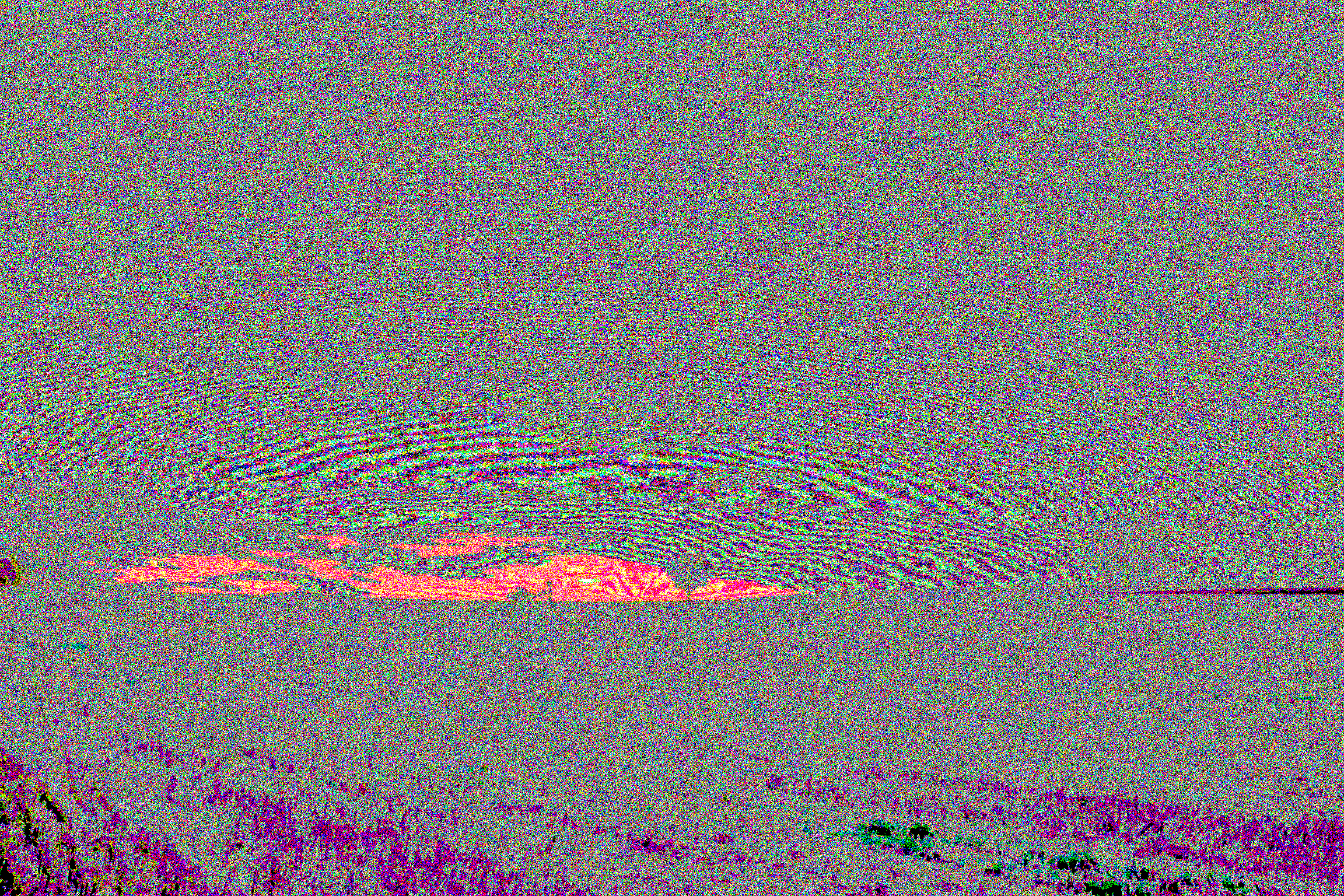
To my eye, there is no apparent banding, like in Frank's image. However, let's be objective. For the following images, I took Frank's and mine and adjusted the histogram for each as indicated in the following table. The purpose of this excercise was to accentuate any banding that might be present by increasing the contrast locally to the bands. This process will also shift the colors so that any potential artifact of monitor settings, graphics card settings, color settings, and the like, will likely affect a different part of the image. The values in the first column represent the part of the histrogram expanded to 0..255.
| Hist. | Frank's Image | My Image |
| 0..63 | 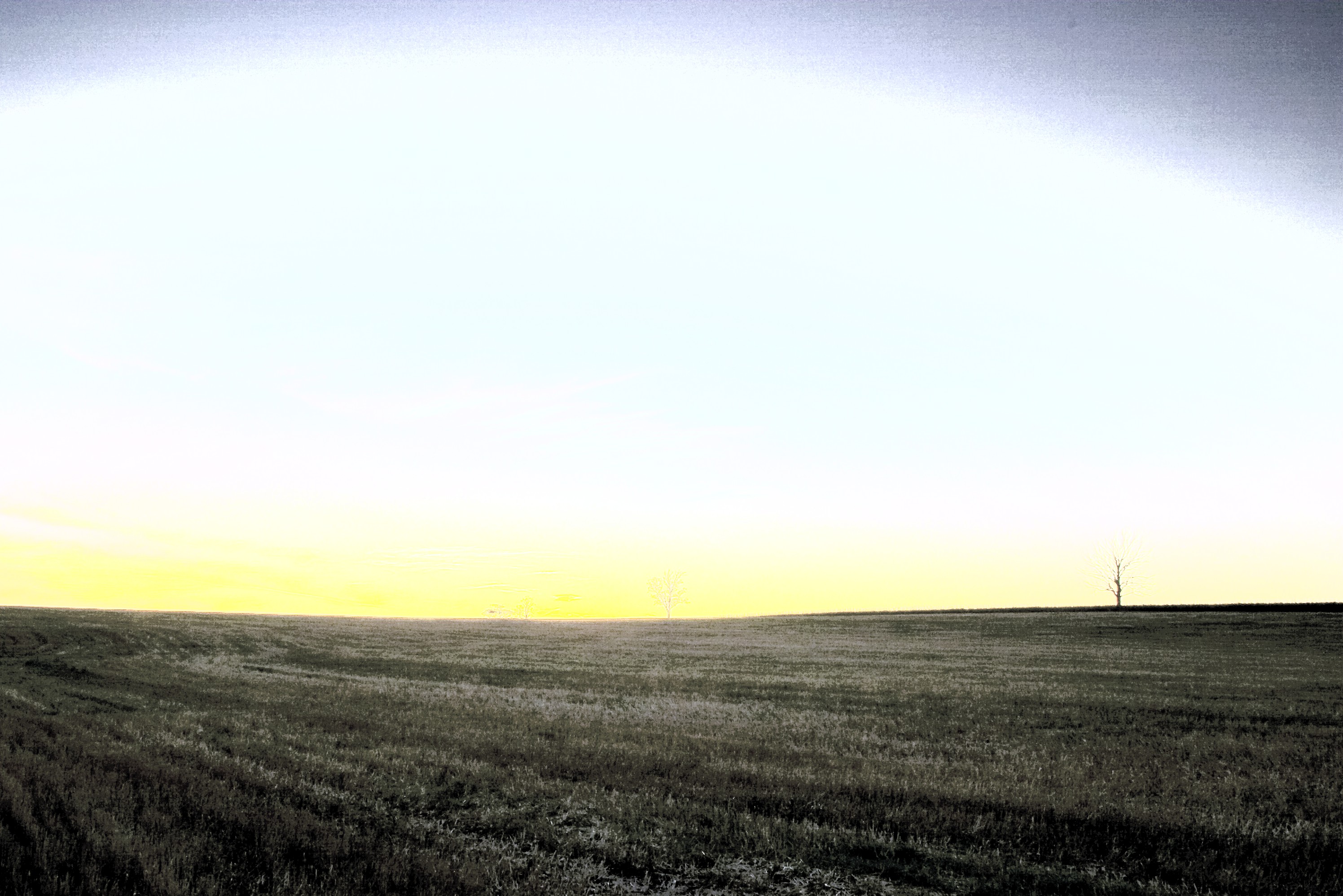 | 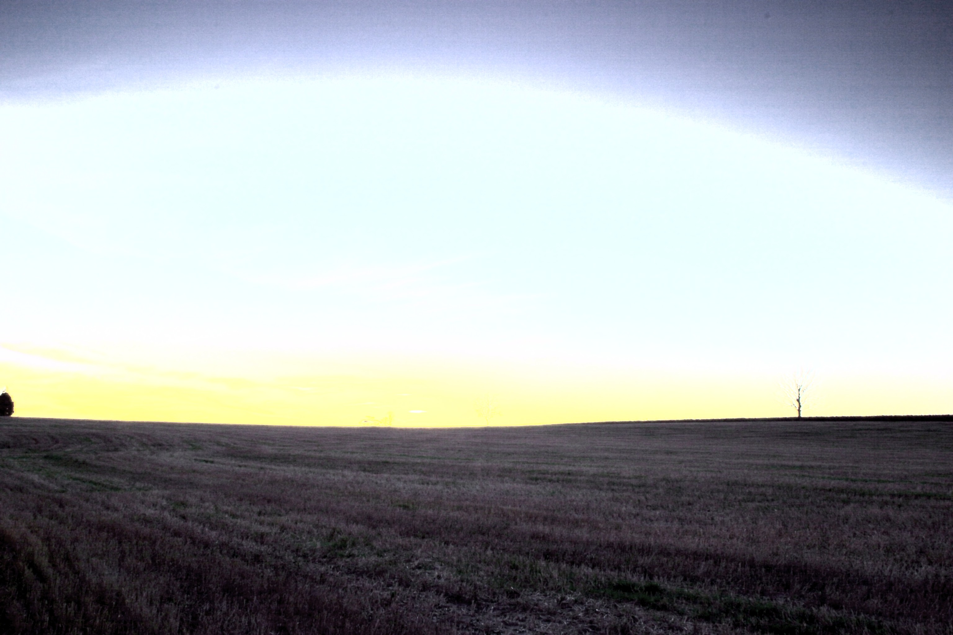 |
| 32..95 | 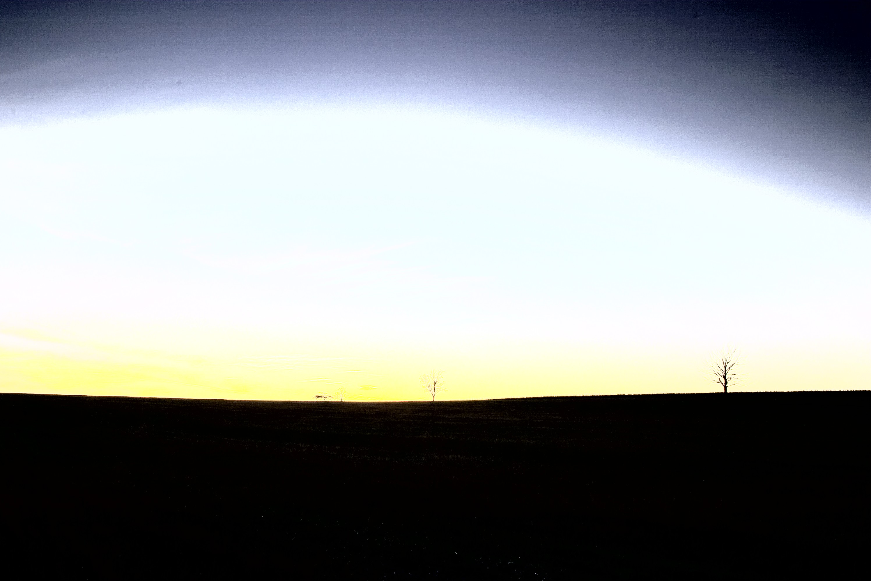 | 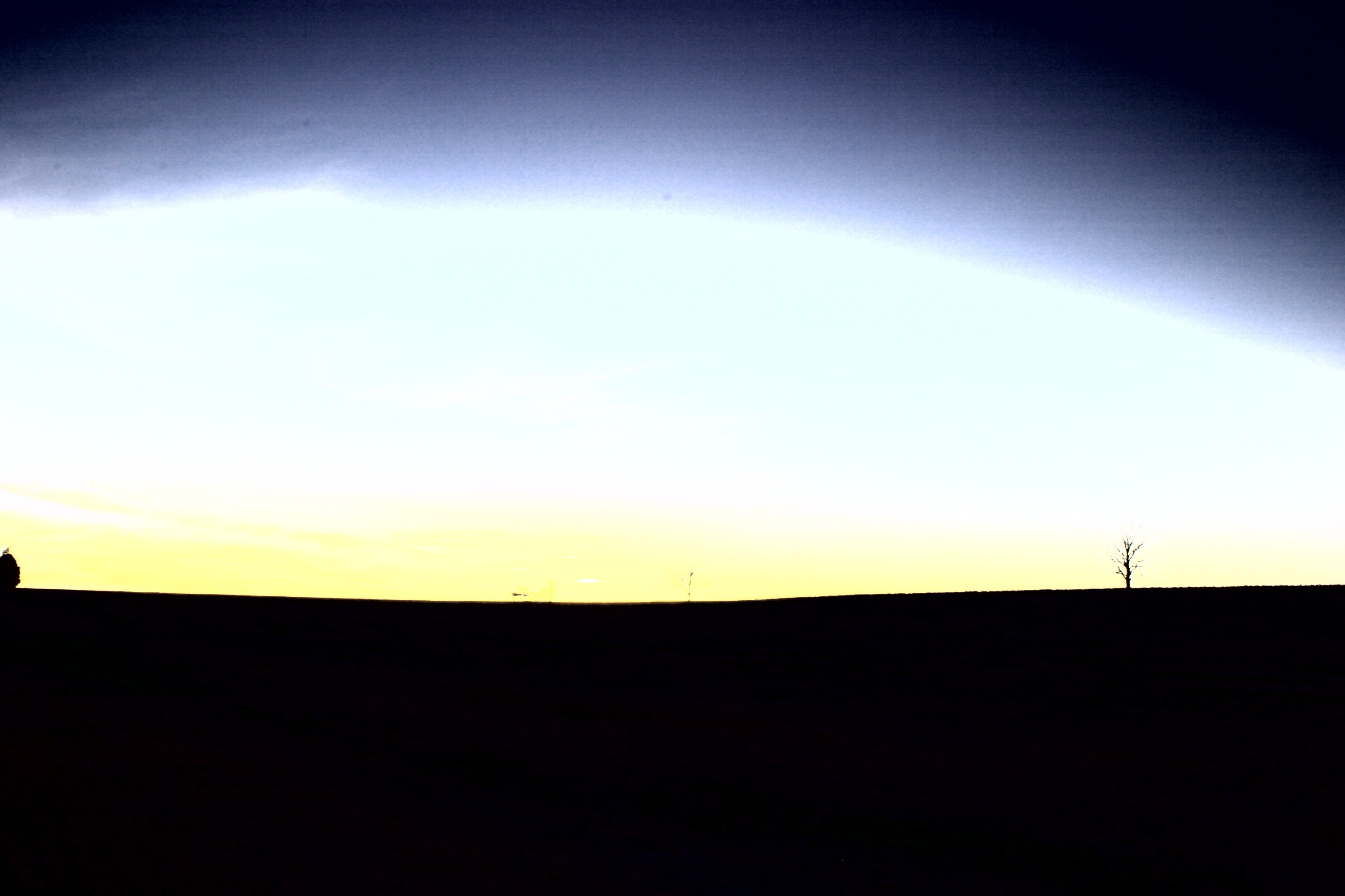 |
| 64..127 | 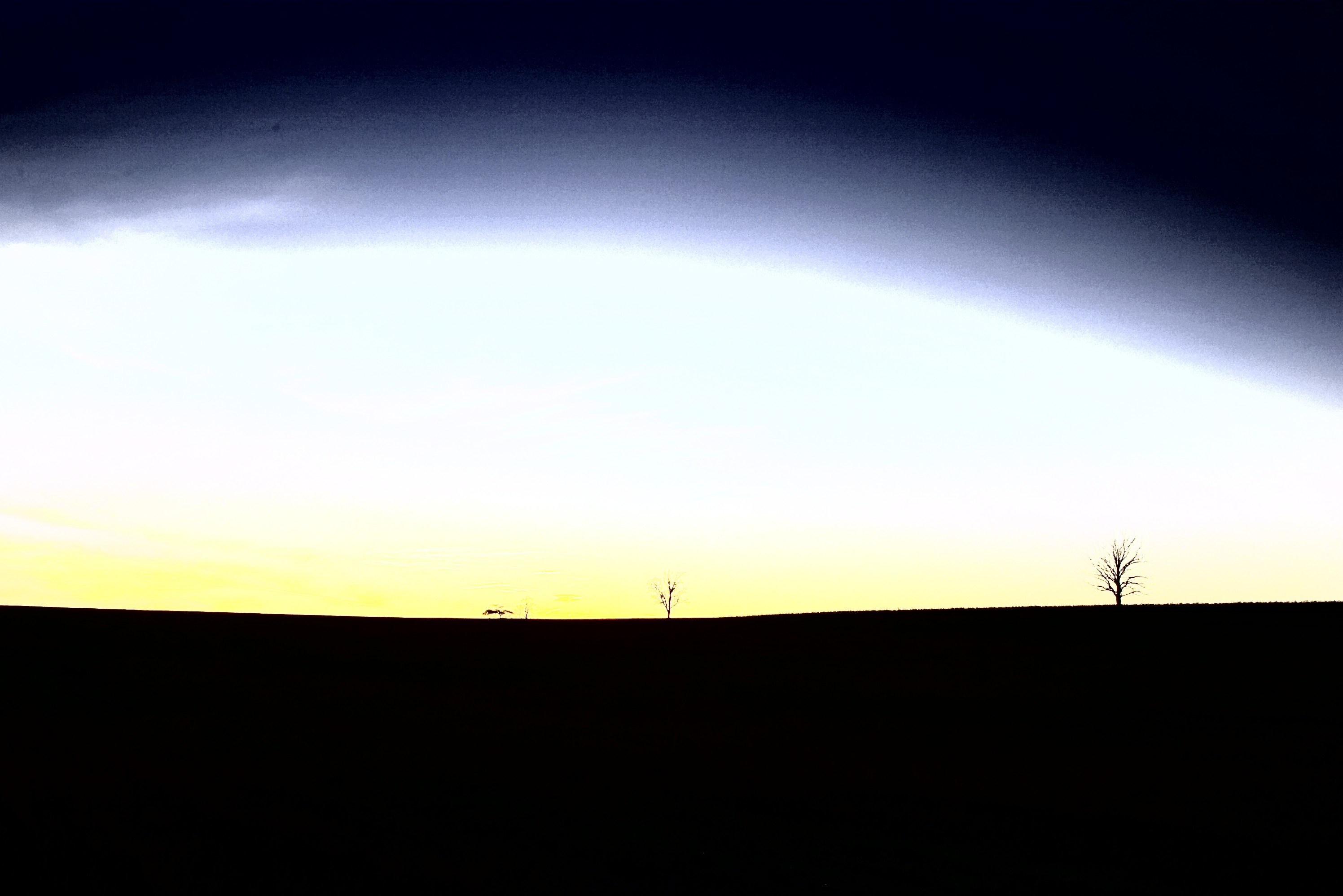 | 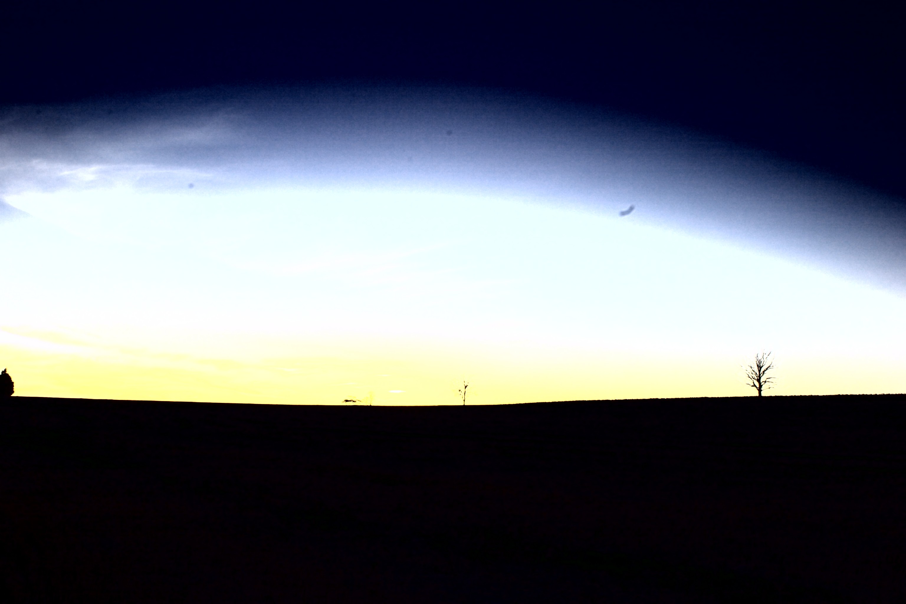 |
| 96..159 | 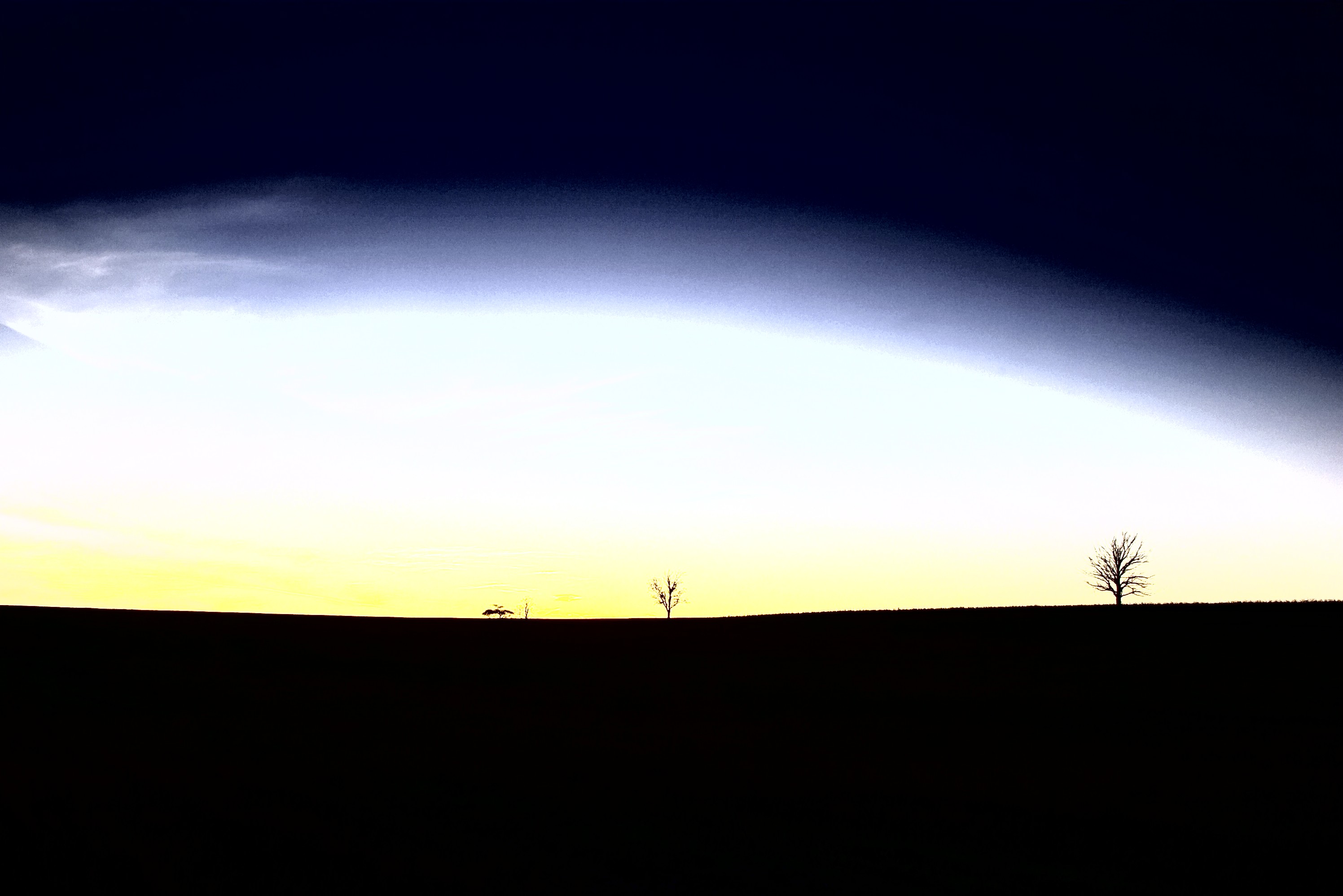 | 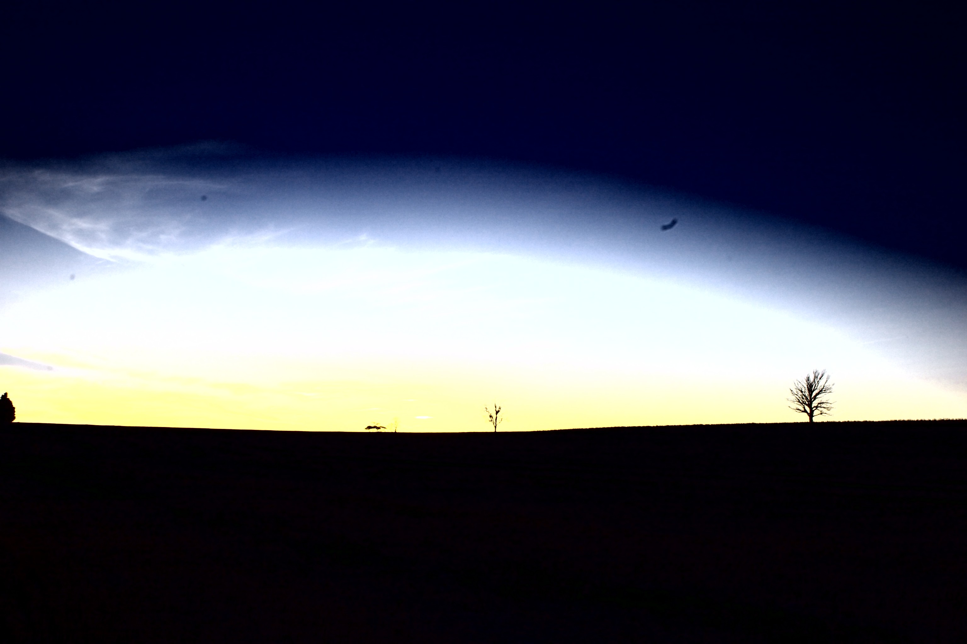 |
| 128..191 | 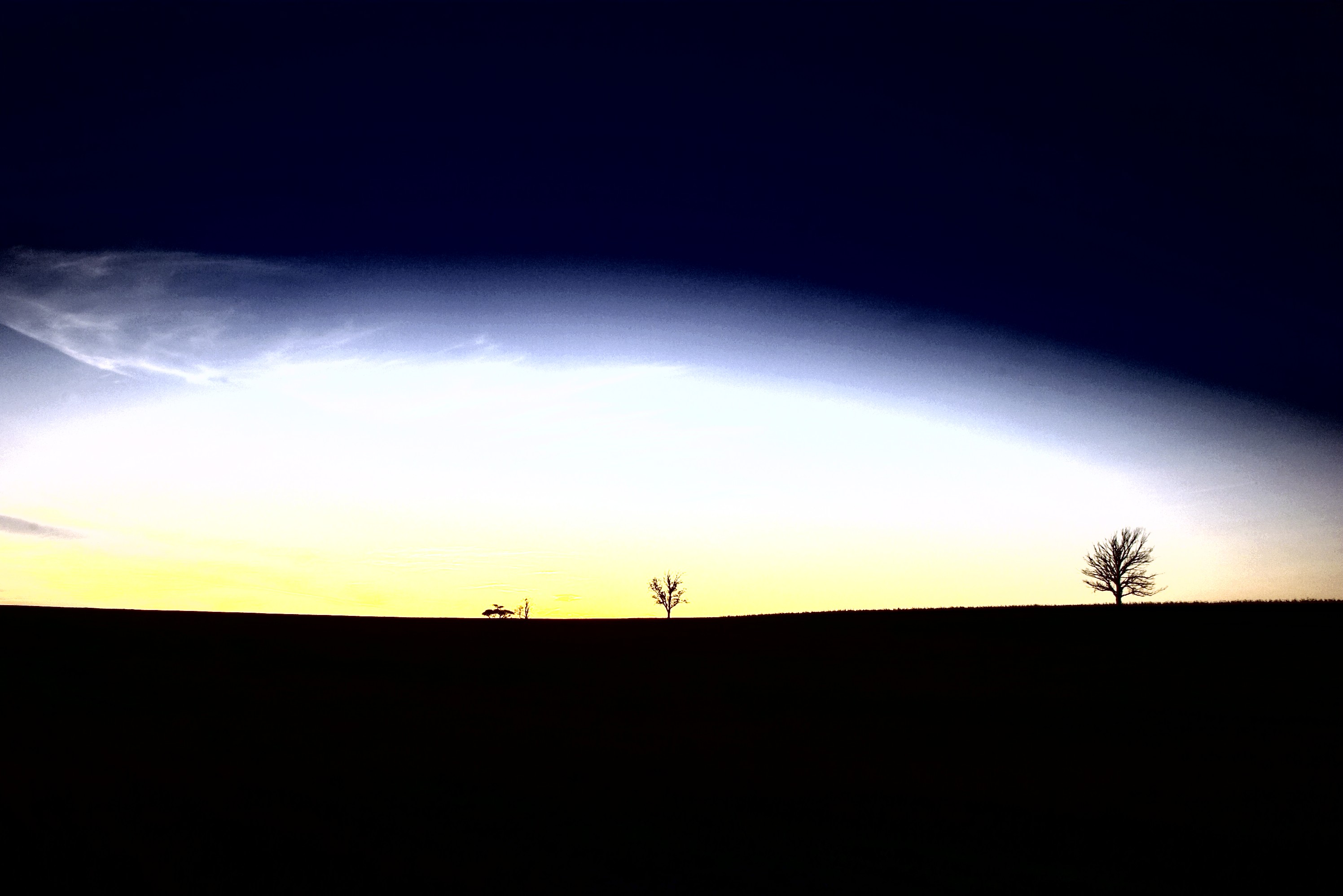 | 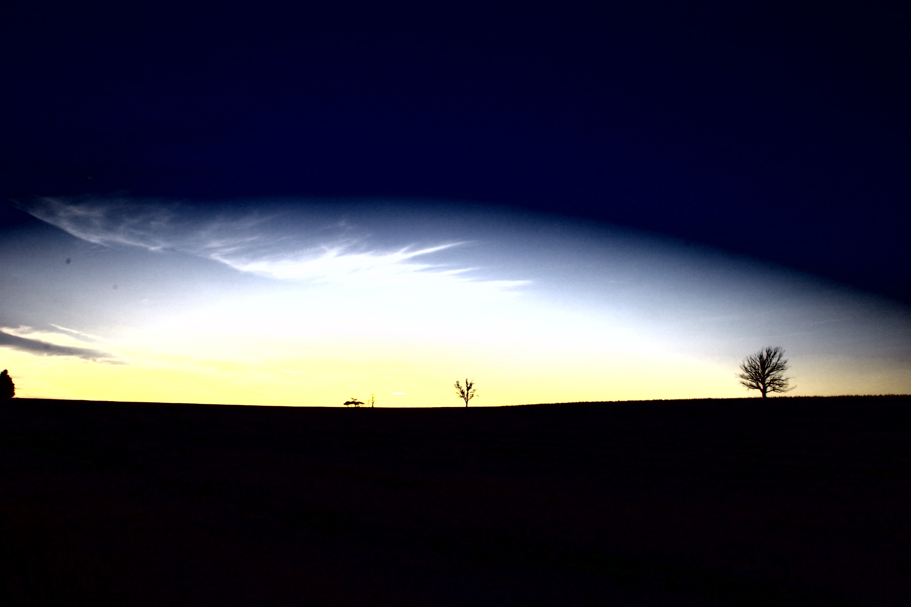 |
| 160..223 | 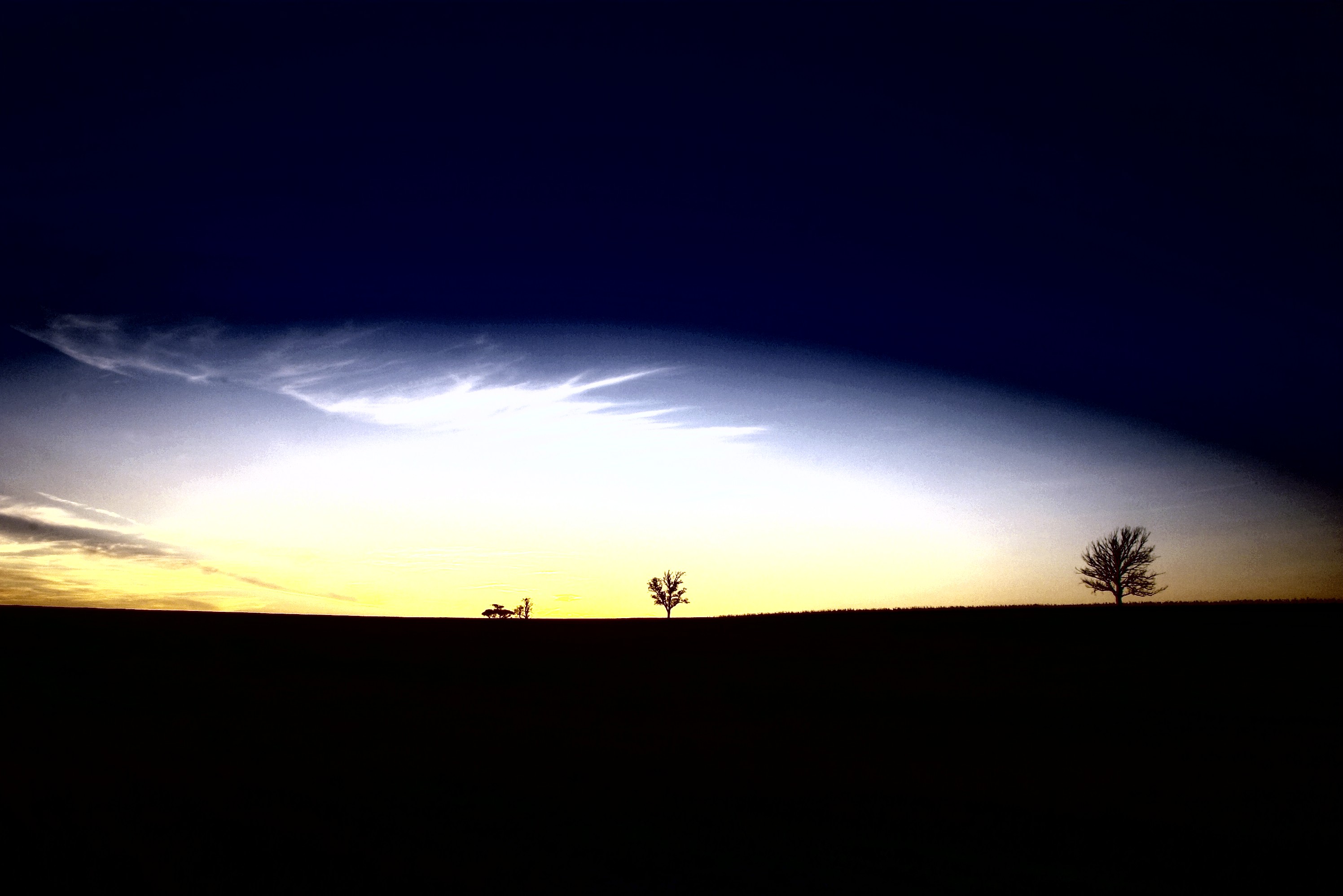 | 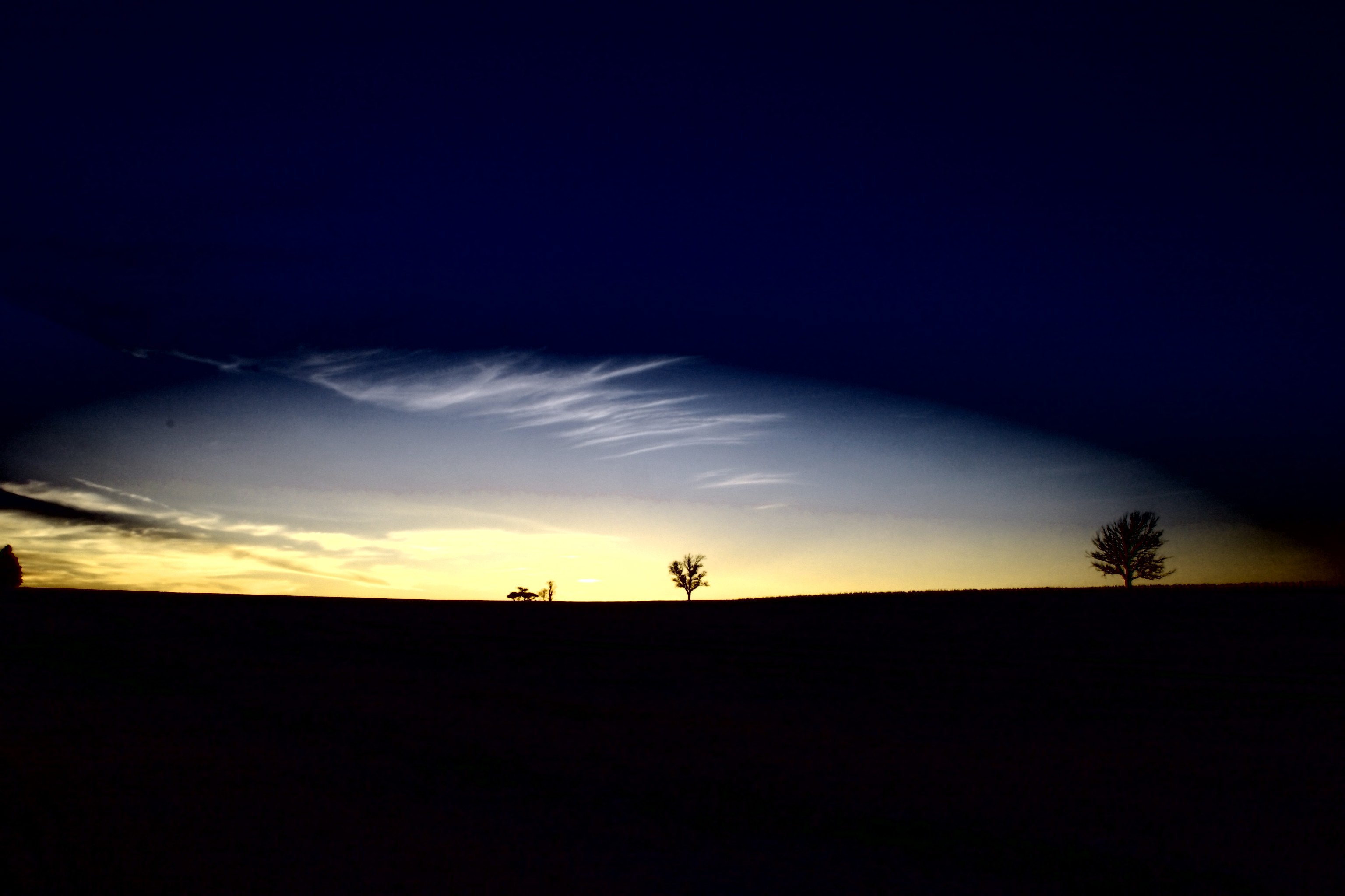 |
| 192..255 | 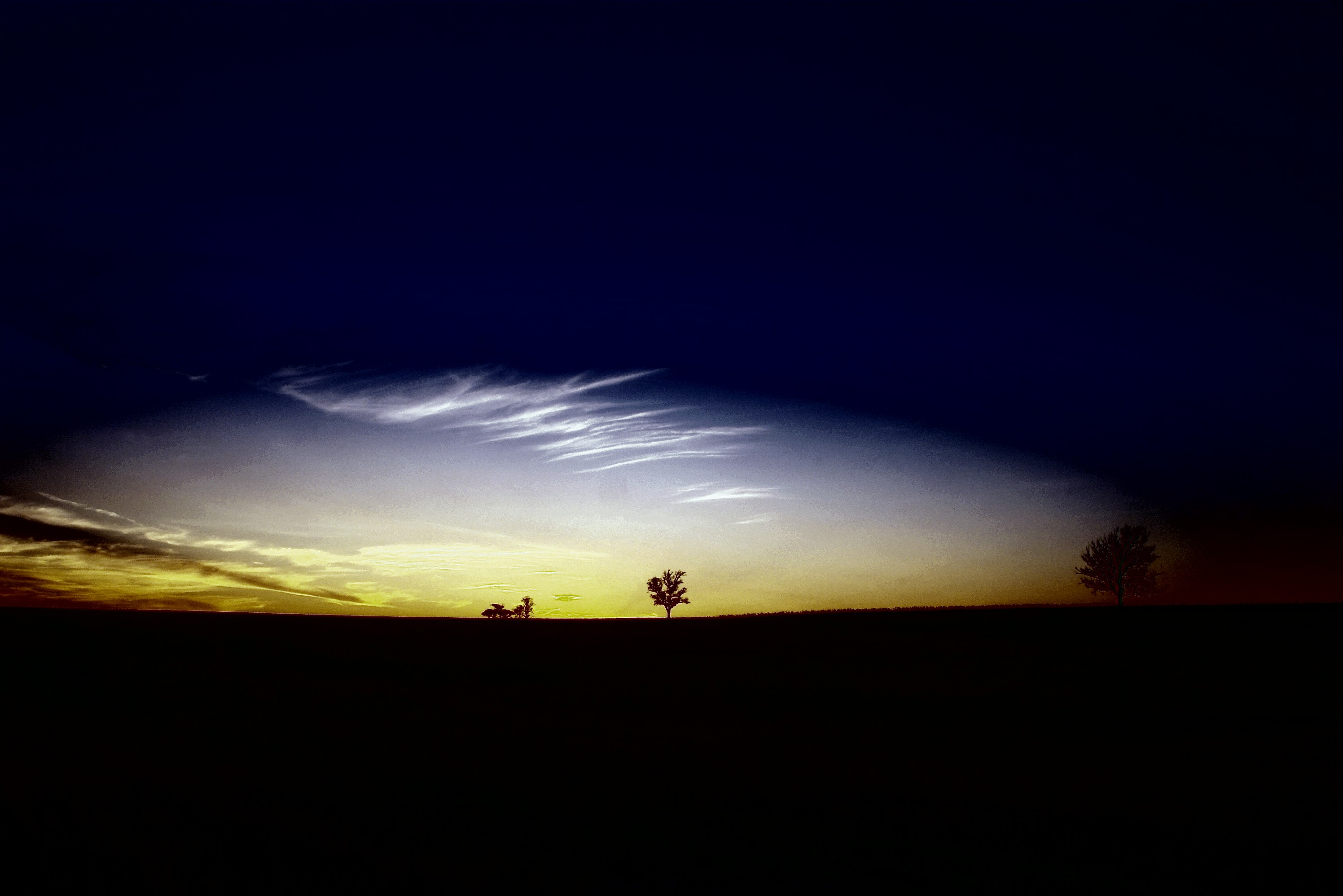 | 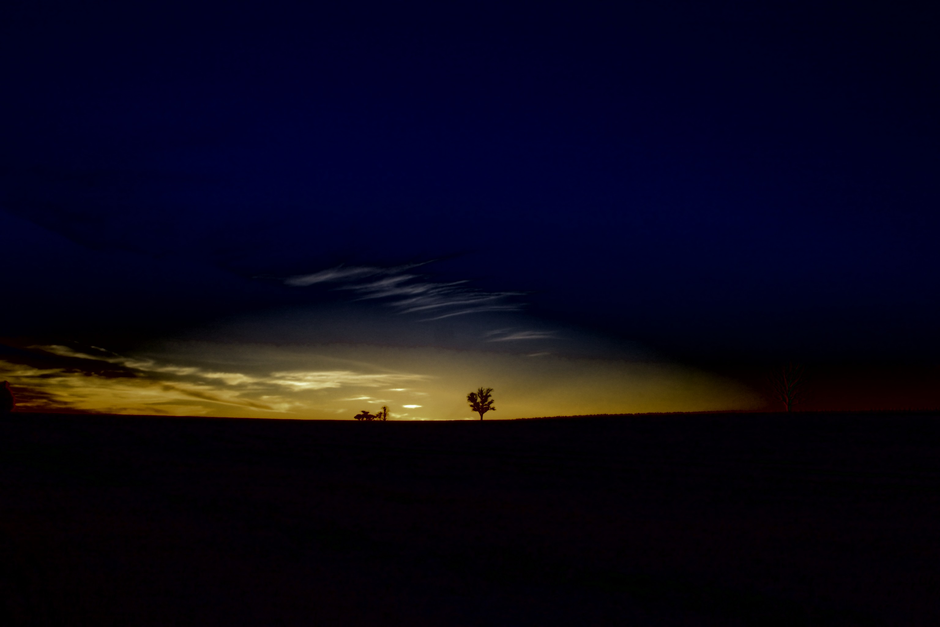 |
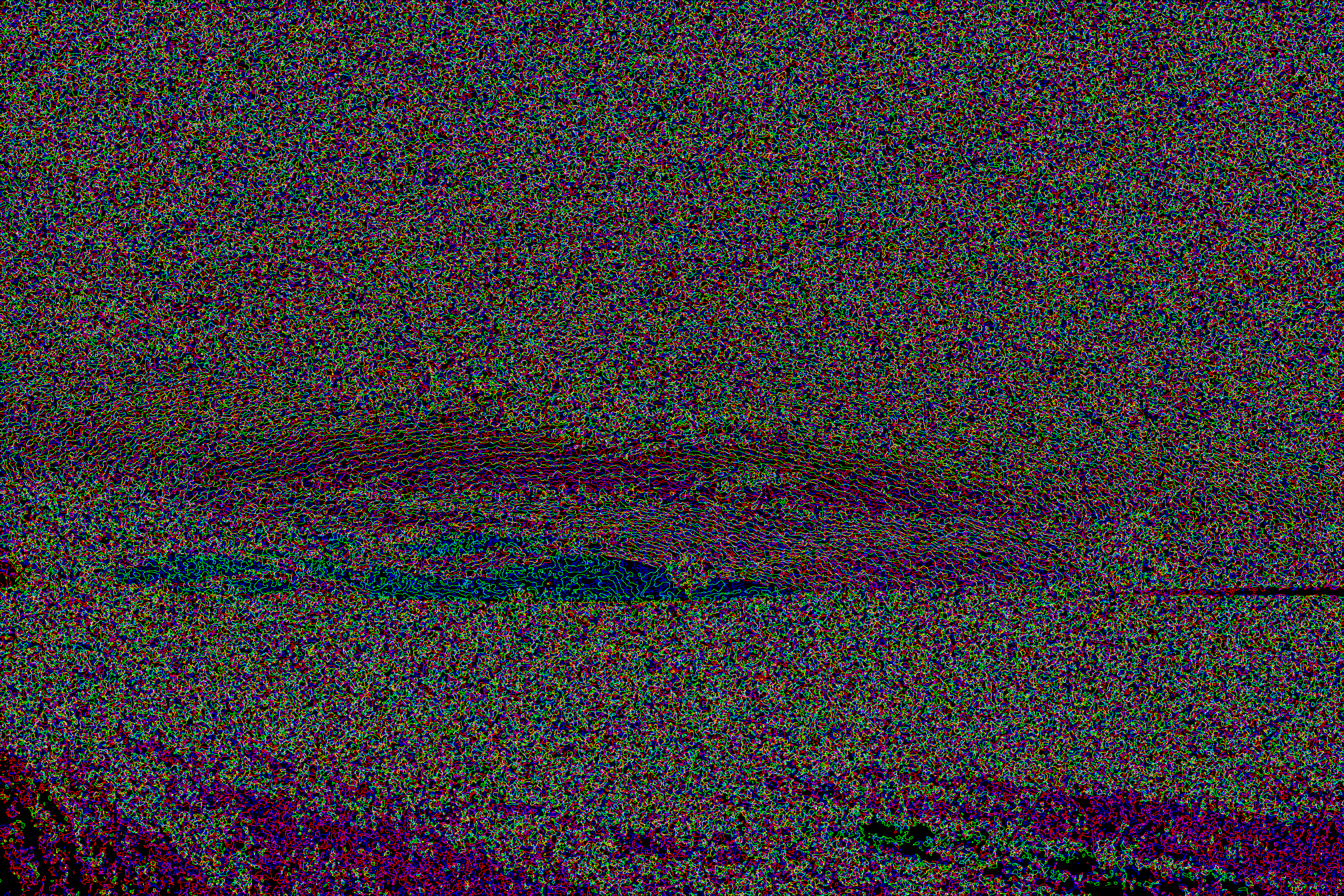
Finally, I created several images to show the boundaries between colors. I used Paintshop Pro 7 for this, because I like the salt and pepper filter, which I used to omit noise and concentrate on the banding pattern. The PSP parameters I used were: Speck size: 3, Sensitivity: 5, Include lower level speck sizes, and aggressive action. I applied this filter in PSP to an image that consisted only of the lowest order bit of each of the RGB channels. I created this image using a filter I wrote to extract a single bitplane.
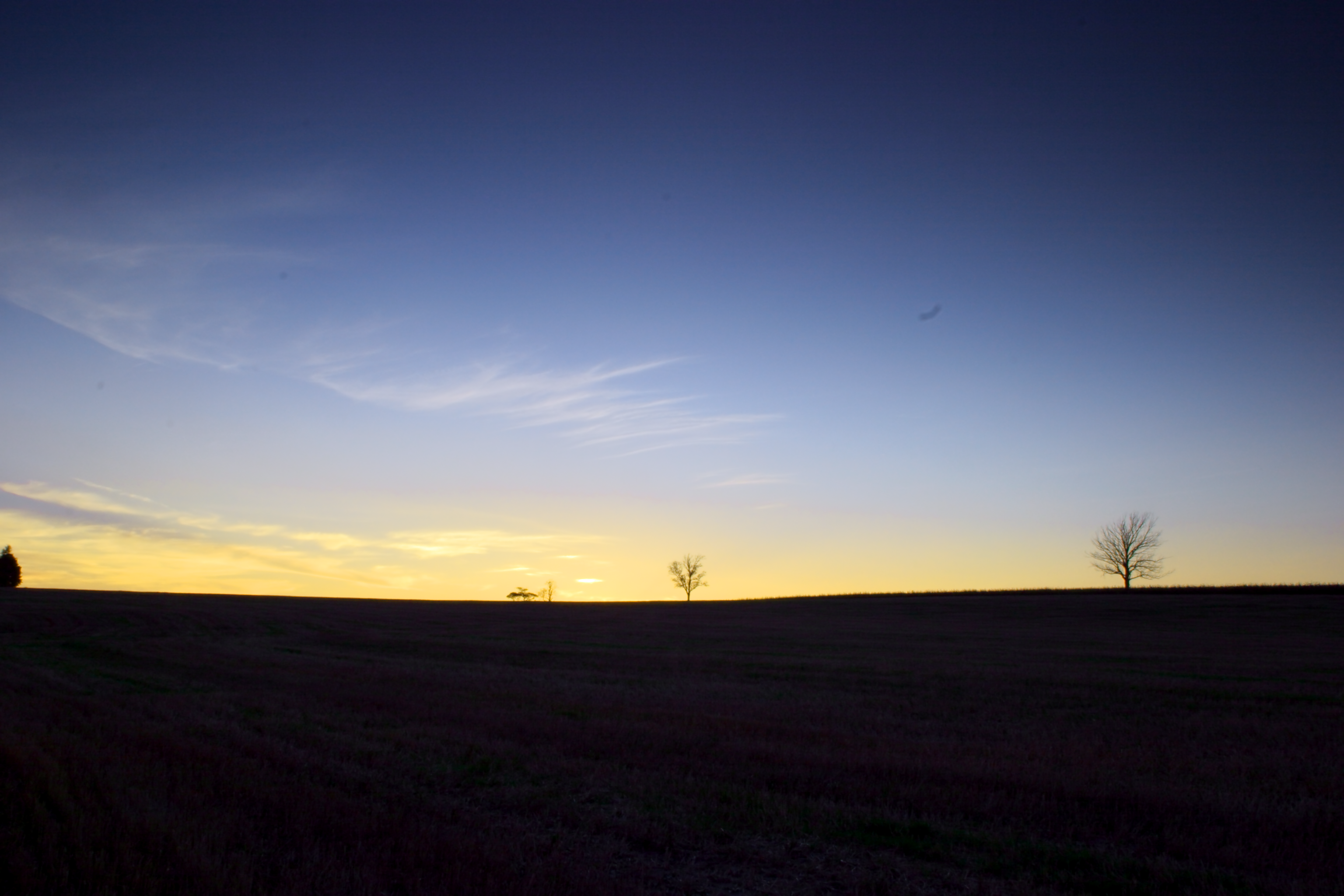
Detail taken from just above horizon on right.
After the salt and pepper filter, I increased the contrast to maximum and then used the edge filter to find the edges. The result is a map that shows the boundaries between neighboring intensities of each of the three channels. I did the same thing with bitplane 7, which should have a frequency about half of bitplane 8, if noise is not the overriding factor.
 Bitplane 8 -- Detail taken from just above horizon on right. |
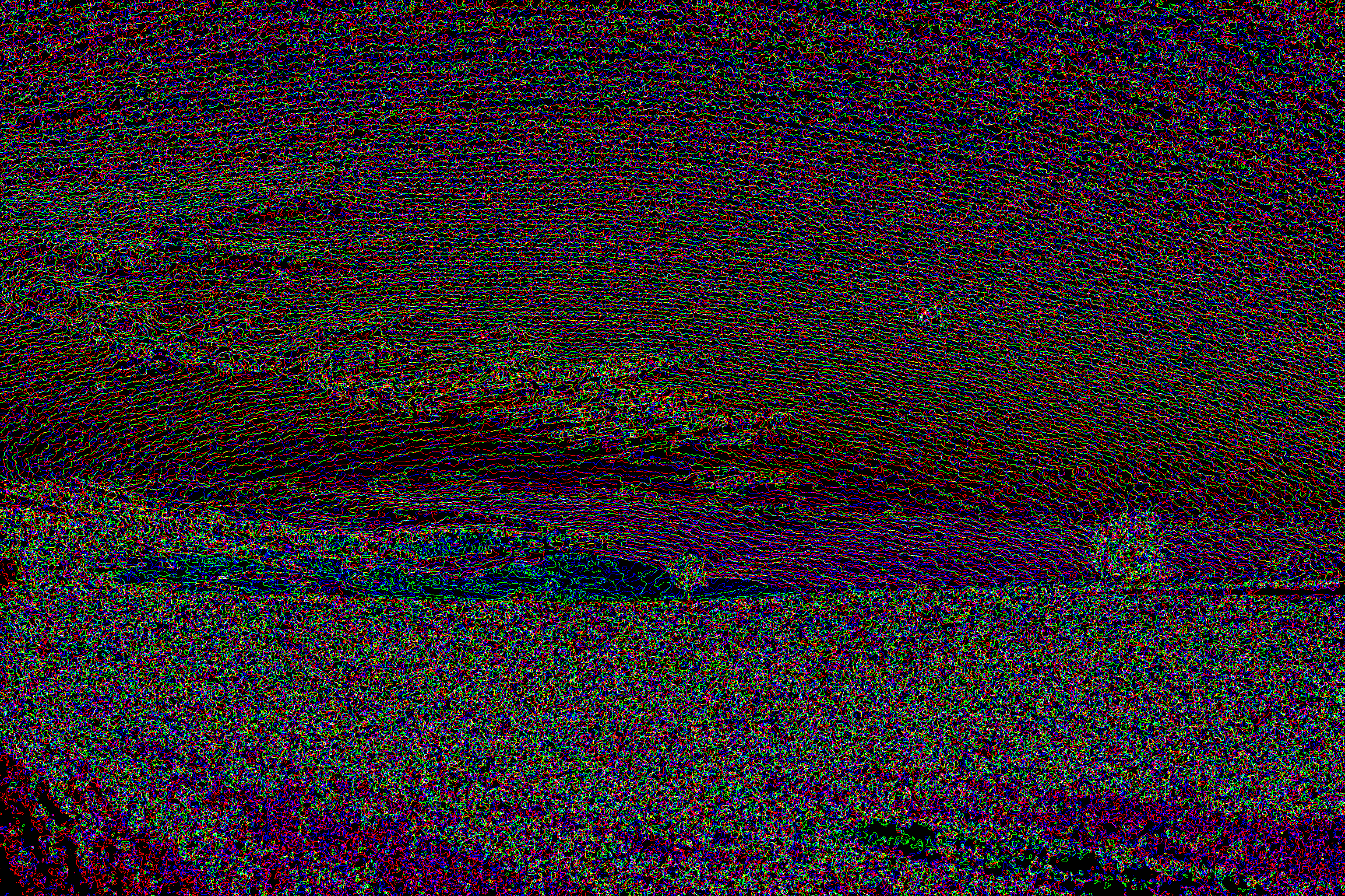 Bitplane 7 -- Detail taken from just above horizon on right. |
If Frank is truly seeing banding in my image, then the locations where he's seeing banding should show up clearly in the image for bitplane 8.
Finally, I combined the edges between intensities, as described above, and combined bitplane 7 and bitplane 8 for each of the three red, green, and blue channels. The dark lines represent bitplane 7 (more significant data), and the grey lines represent bitplane 8 (least significant). If there is no banding, then we would expect in areas where a gradient is present that the dark lines and grey lines would be relatively equally spaced in relation to each other. Furthermore, the grey lines should be more circuitous than the dark bands. If banding IS present, we would expect to see consecutive lines that are either black or grey. Put another way, the bands would come together in the same place.
| Red | 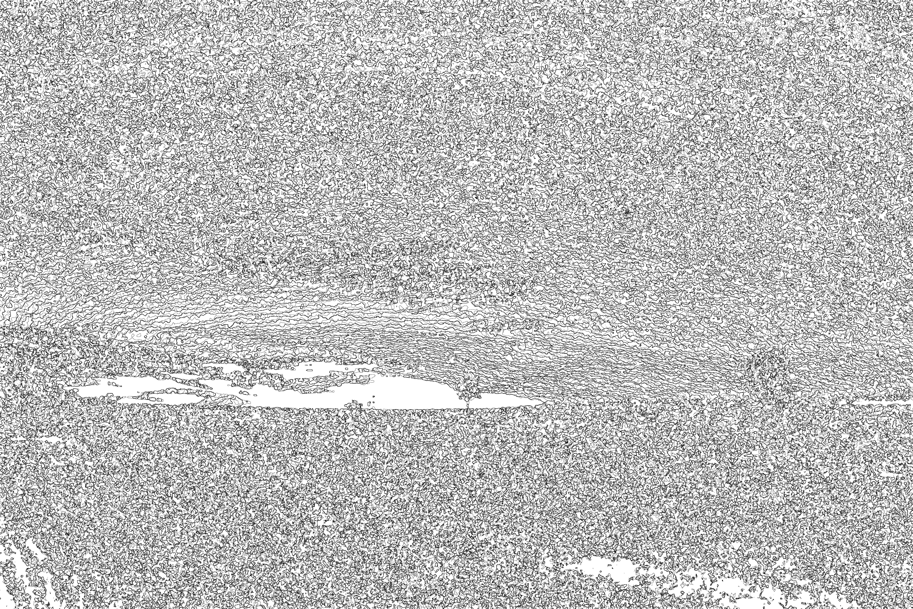 |
| Green | 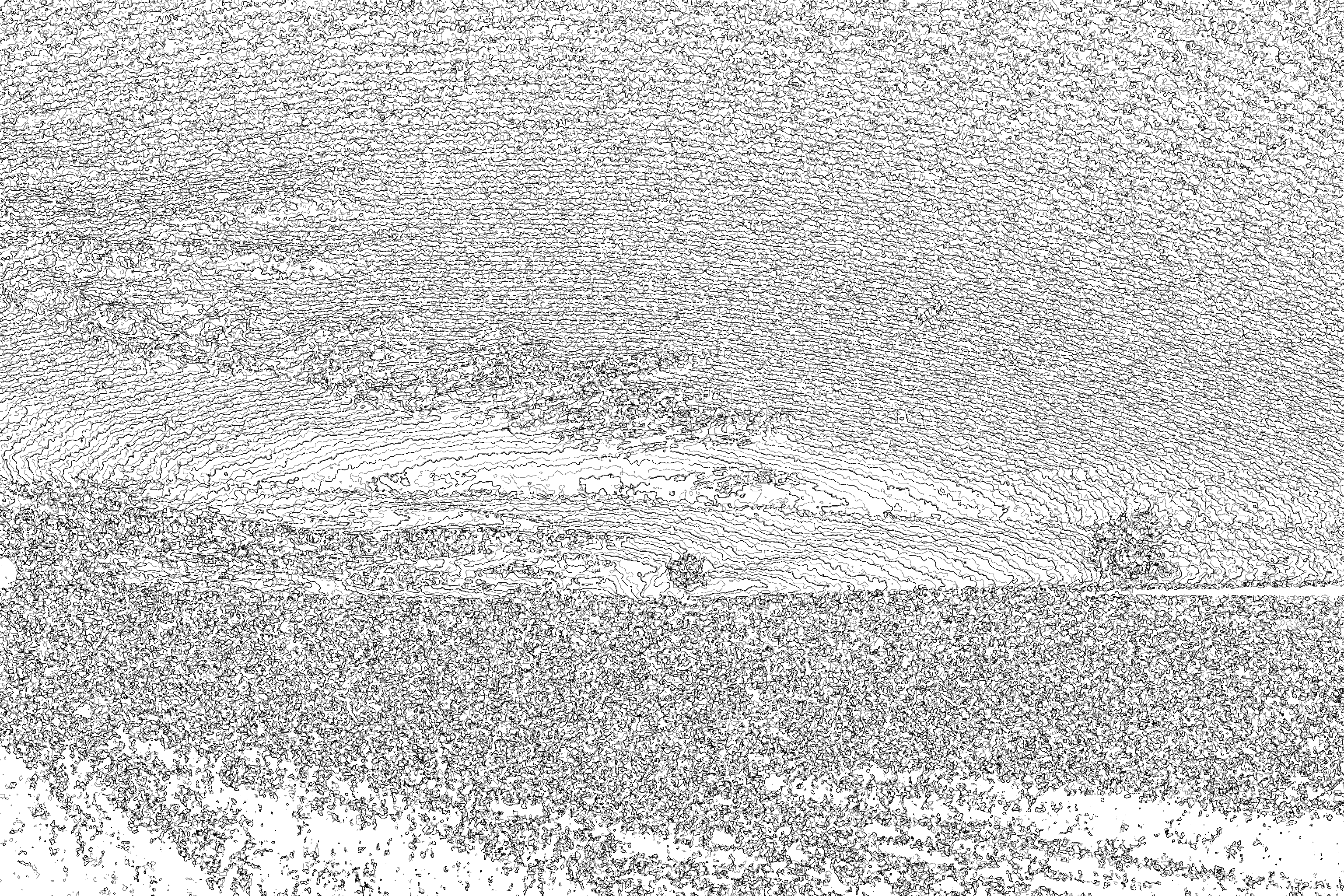 |
| Blue | 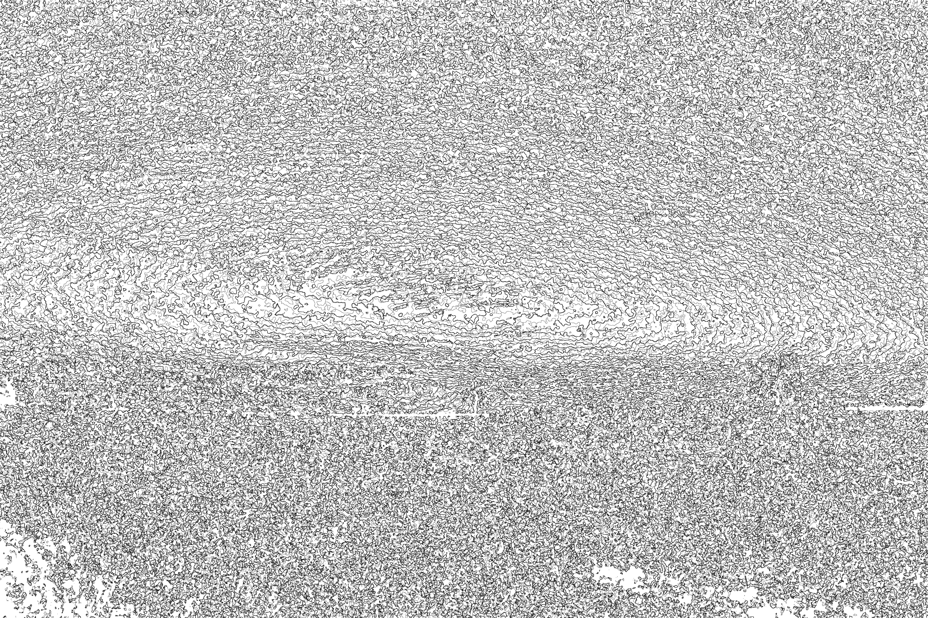 |